Inference

Once the information matrix and information vector have been populated, the path and map can be recovered by the following operation,

The result is a vector, \mu defined over all poses and features, containing the best estimate for each. This operation is very similar to what you encountered before in the simple one-dimensional case, with a bit of added structure. Just as before, all constraints are considered when computing the solution.

Completing the above operation requires solving a system of equations. In small systems, this is an easily realizable task, but as the size of the graph and matrix grows - efficiency becomes a concern.

The efficiency of this operation, specifically the matrix inversion, depends greatly on the topology of the system.

Linear Graph

If the robot moves through the environment once, without ever returning to a previously visited location, then the topology is linear. Such a graph will produce a rather sparse matrix that, with some effort, can be reordered to move all non-zero elements to near the diagonal. This will allow the above equation to be completed in linear time.

Cyclical Graph

A more common topology is cyclical, in which a robot revisits a location that it has been to before, after some time has passed. In such a case, features in the environment will be linked to multiple poses - ones that are not consecutive, but spaced far apart. The further apart in time that these poses are - the more problematic, as such a matrix cannot be reordered to move non-zero cells closer to the diagonal. The result is a matrix that is more computationally challenging to recover.

However, all hope is not lost - a variable elimination algorithm can be used to simplify the matrix, allowing for the inversion and product to be computed quicker.

Variable Elimination

Variable elimination can be applied iteratively to remove all cyclical constraints. Just like it sounds, variable elimination entails removing a variable (ex. feature) entirely from the graph and matrix. This can be done by adjusting existing links or adding new links to accommodate for those links that will be removed.

If you recall the spring analogy, variable elimination removes features, but keeps the net forces in the springs unaltered by adjusting the tension on other springs or adding new springs where needed.

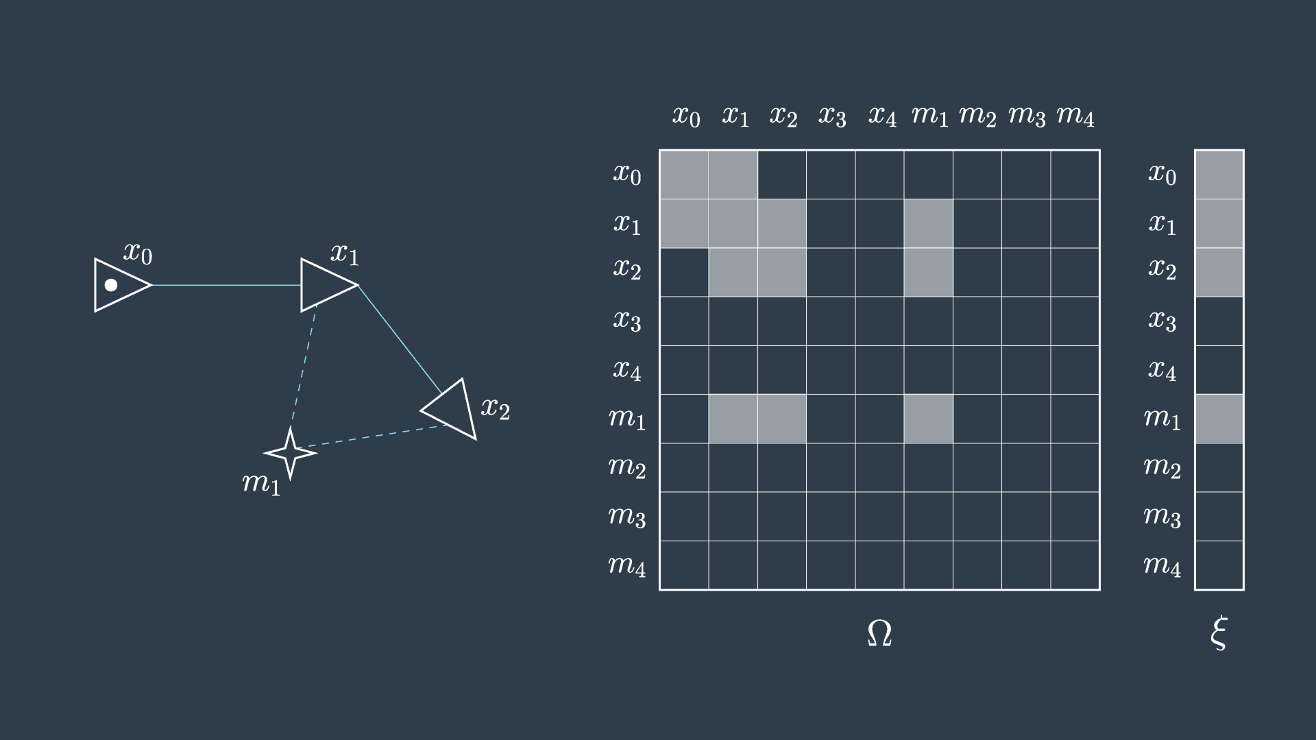
This process is demonstrated in the following two images. The first image shows the graph, matrix, and vector as they were presented in the previous video.

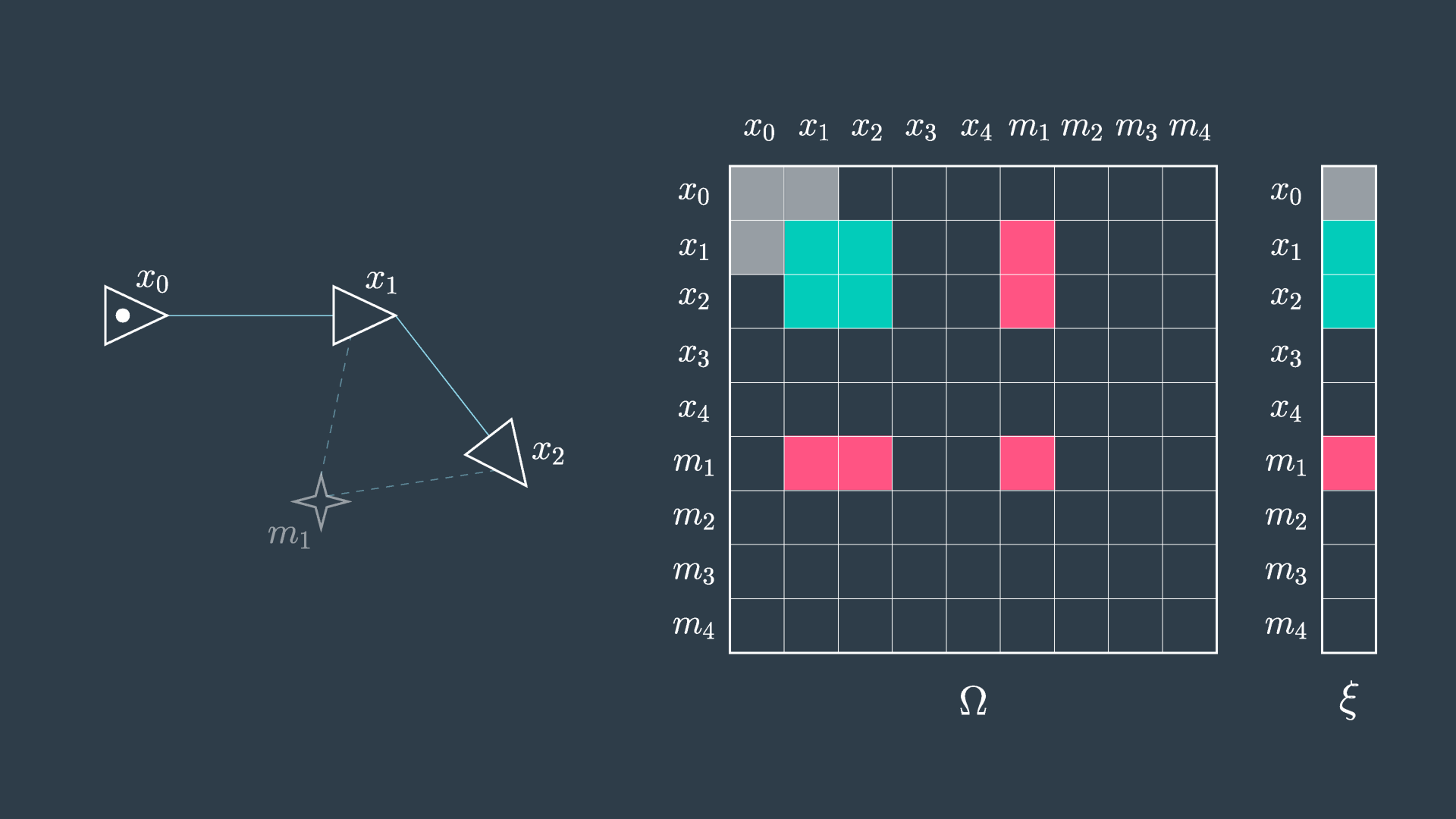
The second image shows the elimination of m_1 . You can see that in this process the matrix will have five cells reset to zero (indicated in red), and four cells will have their values adjusted (indicated in green) to accommodate the variable elimination. Similarly, the information vector will have one cell removed and two adjusted.

This process is repeated for all of the features, and in the end the matrix is defined over all robot poses. At this point, the same procedure as before can be applied, \mu = \Omega^{-1}\xi .

Performing variable elimination on the information matrix/vector prior to performing inference is less computationally intense than attempting to solve the inference problem directly on the unaltered data.

In practice, the analytical inference method described above is seldom applied, as numerical methods are able to converge on a sufficiently accurate estimate in a fraction of the time. More will be said on this topic later, but first it is important to explore how nonlinear constraints are handled in GraphSLAM.